In class exercise 6

#1 Load Data

pacman::p_load(sf, sfdep, tmap, tidyverse)

Let’s start by importing Geospatial data

hunan <- st_read(dsn = "data/geospatial", 
                 layer = "Hunan")

Reading layer `Hunan' from data source 
  `/Users/keredpoh/Desktop/keredpoh/IS415-GAA/In-class_Ex/In-class_Ex06/data/geospatial' 
  using driver `ESRI Shapefile'
Simple feature collection with 88 features and 7 fields
Geometry type: POLYGON
Dimension:     XY
Bounding box:  xmin: 108.7831 ymin: 24.6342 xmax: 114.2544 ymax: 30.12812
Geodetic CRS:  WGS 84

Next, Aspatial data

hunan2012 <- read_csv("data/aspatial/Hunan_2012.csv")

hunan_GDPPC <- left_join(hunan, hunan2012) %>%
  select(1:4, 7,  15)

#2 Visualising plot

tmap_mode("plot")

tm_shape(hunan_GDPPC) +
  tm_fill("GDPPC",
          style = "quantile",
          palette = "Blues",
          title = "GDPPC") +
  tm_layout(main.title =  "Distribution of GDP per capita by distribution",
  main.title.position = "center",
  main.title.size = 0.9,
  legend.height = 0.45,
  legend.width = 0.35,
  frame = TRUE) +
  tm_borders(alpha = 0.5) +
  tm_compass(type = "8star", size = 2) +
  tm_scale_bar() +
  tm_grid(alpha = 0.2)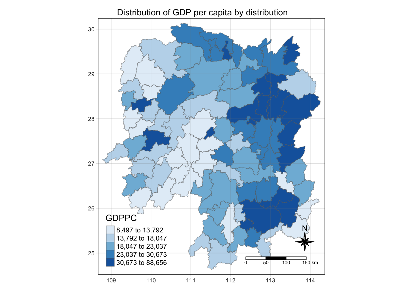

#3 Computing using different Contiguity neighbour methods

queen method

cn_queen <- hunan_GDPPC %>%
  mutate(nb = st_contiguity(geometry),
         .before = 1)

rook method

cn_rook <- hunan_GDPPC %>%
  mutate(nb = st_contiguity(geometry),
         queen = FALSE,
         .before = 1)

#4 Contiguity weights queen method

wm_q <- hunan_GDPPC %>%
  mutate(nb = st_contiguity(geometry),
         wt = st_weights(nb),
         .before = 1)