Show code
pacman::p_load(sf, tmap, tidyverse)#Installing and loading packages
pacman::p_load(sf, tmap, tidyverse)NGA_wp <- read_rds("data/rds/NGA_wp.rds")p1 <- tm_shape(NGA_wp) +
tm_fill("wp_functional",
n= 10,
style = "equal",
palette ="Blues") +
tm_borders(lwd = 0.1,
alpha = 1) +
tm_layout(main.title = "Distribution of functional water",
legend.outside = FALSE)
# n = 10 indicates 10 range of colors
# style = equal indicates the distribution of data, in this case, equal refers to equal difference per range as per seen in the plotp2 <- tm_shape(NGA_wp) +
tm_fill("total_wp",
n= 10,
style = "equal",
palette ="Blues") +
tm_borders(lwd = 0.1,
alpha = 1) +
tm_layout(main.title = "Distribution of total water point",
legend.outside = FALSE)Arrange both maps into 1 visualisation
tmap_arrange(p2, p1, nrow = 1)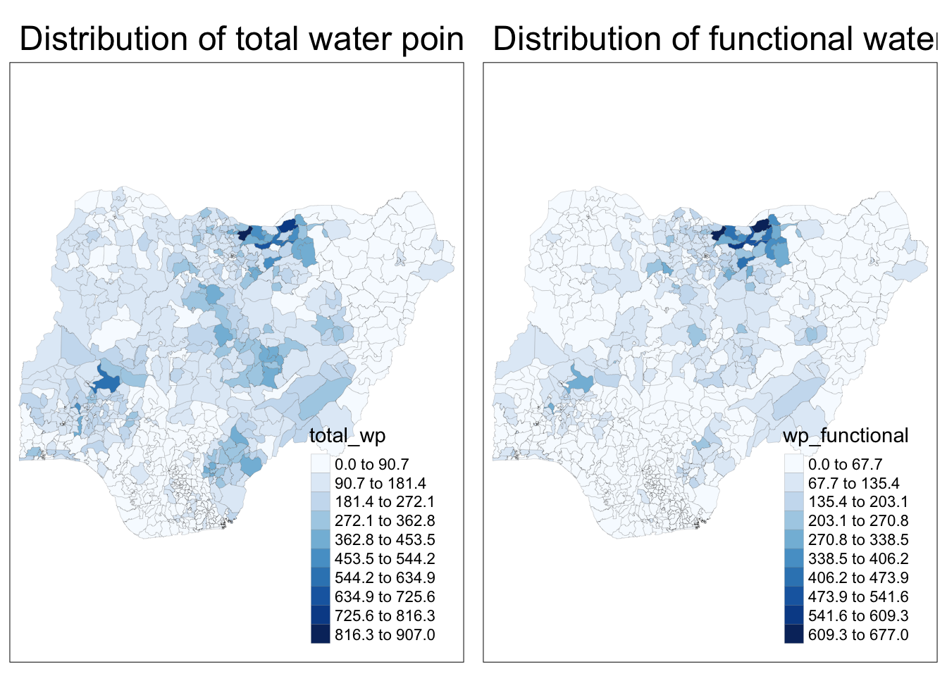
NGA_wp <- NGA_wp %>%
  mutate(pct_functional = wp_functional/total_wp) %>%
mutate(pct_non_functional = wp_nonfunctional/total_wp)p3 <- tm_shape(NGA_wp) +
tm_fill("pct_functional",
n = 10,
style = "equal",
palette = "Blues") +
tm_borders(lwd= 0.1,
alpha = 1) +
tm_layout(main.title = "Distribution of Proportion of\nFunctional WaterPoints",
legend.outside = FALSE)
p4 <- tm_shape(NGA_wp) +
tm_fill("pct_non_functional",
n = 10,
style = "equal",
palette = "Blues") +
tm_borders(lwd= 0.1,
alpha = 1) +
tm_layout(main.title = "Distribution of Proportion of\nNon_Functional WaterPoints",
legend.outside = FALSE)
tmap_arrange(p4, p3, nrow = 1)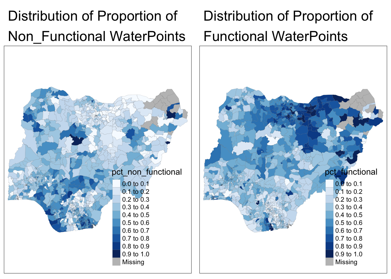
Step 1: Exclude records with NA
NGA_wp <- NGA_wp %>%
  drop_na()
Step 2: Creating customised classification
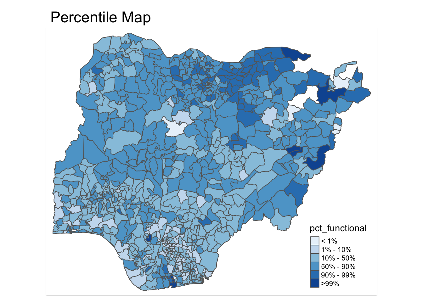
percent <- c(0,.01,.1,.5,.9,.99,1)
var <- NGA_wp["pct_functional"] %>%
  st_set_geometry(NULL)
quantile(var[,1], percent)
0% 1% 10% 50% 90% 99% 100%
0.00000000 0.01818182 0.18181818 0.41666667 0.76086957 1.00000000 1.00000000 # NULL forces NGA_wp["pct_functional"] into var (dataframe)get.var <- function(vname, df) {
v <- df[vname] %>%
st_set_geometry(NULL)
v <- unname(v[,1])
return(v)
}percentmap <- function(vnam, df, legtitle=NA, mtitle = "Percentile Map"){
percent <- c(0,.01,.1,.5,.9,.99,1)
var <- get.var(vnam, df)
bperc <- quantile(var, percent)
tm_shape(df) +
tm_polygons() +
tm_shape(df) +
tm_fill(vnam,
title = legtitle,
breaks=bperc,
palette="Blues",
labels = c("< 1%","1% - 10%", "10% - 50%", "50% - 90%", "90% - 99%", ">99%")) +
tm_borders() +
tm_layout(main.title = mtitle,
title.position = c("right", "bottom"))
}
percentmap("pct_functional", NGA_wp,)